🚌 Data Analytics Mini Project 1🚉

Author: Mike Ee, mikeee.co

A. Introduction

As part of the Singapore Land Transport Masterplan (LTMP) 2040's Walk-Cycle-Ride goals, there is a strong desire to strive for greater multi-modal journeys (i.e. bus-train transfers).

Research Question (RQ):

How does bus passenger load vary in the north eastern corridor of Singapore, specifically at the Kovan-Serangoon-Woodleigh region, and what does the concentration of passenger load suggest about bus-rail integration stated in LTMP 2040?

B. Data profiling & munging

🤦🏻Error in retrieving first query due to typo error in API key (i.e. additional E)

import requests

headers = {"AccountKey": account_key.strip("~~~~E"), "accept": "application/json"} response = requests.get("https://datamall2.mytransport.sg/ltaodataservice/BusStops", headers=headers)

print(response.status_code) print(response.json()) # Prints results as one chunk ~ difficult to read

1. Retrieving Bus Stop dataset from Sg Land Transport Authority Datamall

import requests
import json
import pandas as pd
!pip install python-dotenv

from dotenv import load_dotenv
import os

load_dotenv()

account_key = os.environ["LTA_ACCOUNT_KEY"]
onemap_email = os.environ["ONEMAP_EMAIL"]
onemap_password = os.environ["ONEMAP_PASSWORD"]

headers = {"AccountKey": account_key, "accept": "application/json"}
response = requests.get("https://datamall2.mytransport.sg/ltaodataservice/BusStops", headers=headers)

# Check Status Code Query (200 = OK)
print(f"Query Status Code: {response.status_code}")

# Check number of records being returned in call
print(f"Number of records: {len(response.json()['value'])}")

# Print results in more readable JSON format
#print(json.dumps(response.json(), indent=2))

Requirement already satisfied: python-dotenv in c:\users\micha\anaconda3\lib\site-packages (1.1.0)

Query Status Code: 200
Number of records: 500

2. Coding pagination to ensure all entries in server dataset are called

# Varible to store all entries (think of adding garlic to an empty bowl)
all_records = []  
skip = 0

while True:                                      # $skip suggested from API docu
    url = f"{"https://datamall2.mytransport.sg/ltaodataservice/BusStops"}?$skip={skip}"             
    response = requests.get(url, headers=headers)
    batch = response.json().get("value", [])
    
    if len(batch) == 0:                          # stop once garlic is gone
        break
    
    all_records.extend(batch)                    # add garlic clove to bowl
    
    if len(batch) < 500:                         # last clove - stop
        break
    
    skip += 500                                  # move to next clove

df = pd.DataFrame(all_records)                   # storing all records as a new df

df

	BusStopCode	RoadName	Description	Latitude	Longitude
0	01012	Victoria St	Hotel Grand Pacific	1.296848	103.852536
1	01013	Victoria St	St. Joseph's Ch	1.297710	103.853225
2	01019	Victoria St	Bras Basah Cplx	1.296990	103.853022
3	01029	Nth Bridge Rd	Opp Natl Lib	1.296673	103.854414
4	01039	Nth Bridge Rd	Bugis Cube	1.298208	103.855491
...	...	...	...	...	...
5200	99139	Changi Village Rd	Blk 5	1.388195	103.987234
5201	99161	Nicoll Dr	Aft Changi Beach CP 3	1.390303	103.992975
5202	99171	Nicoll Dr	Changi Beach CP 2	1.391161	103.990992
5203	99181	Telok Paku Rd	Bef S'pore Aviation Ac	1.387793	103.988393
5204	99189	Telok Paku Rd	S'pore Aviation Ac	1.388414	103.989716

5205 rows × 5 columns

Observation 🤔

• Made a total of 11 calls for Bus Stop dataset, 10 full batches of 500

3. Coding API call for Passenger Volume by Bus Stop CSV download link

headers = {"AccountKey": account_key, "accept": "application/json"}
response = requests.get("https://datamall2.mytransport.sg/ltaodataservice/PV/Bus", headers=headers)

# Check Status Code Query (200 = OK)
print(f"Query Status Code: {response.status_code}")

# Check number of records being returned in call
print(f"Number of records: {len(response.json()['value'])}")

Query Status Code: 200
Number of records: 1

# Importing the io module, a Python lib that provides core tools for working with streams - objs tt rep 
# data sources or destinations (e.g. files, in-memory buffers, or network connections.ta sources or destinations, 
# such as files, in-memory buffers, or network connections.
import io
# zipfile module necy for extracting python-ready data from zipped files
import zipfile 

# Extract temp dl URL from JSON metadata
api_data = response.json().get("value", [])

if api_data:
# Retrieve URL from the 'Link' key of the first record 
#(in this case there is only 1 record as indicated by API docu)
    actual_download_url = api_data[0].get("Link")
    print(f"Download Link Found: {actual_download_url.split('?')[0]}?[REDACTED]")

# Create a header mimicking a standard web browser for script to appear human
# so that it can gain entry into Amazon S3 cloud server to access dataset
# Without this line, returns 403 Forbidden
    download_headers = {
    "User-Agent": "Mozilla/5.0 (Windows NT 10.0; Win64; x64) AppleWebKit/537.36 (KHTML, like Gecko) Chrome/120.0.0.0 Safari/537.36"
}

# Request dl of zip file content with the headers attached
    file_response = requests.get(actual_download_url, headers=download_headers)
    
    if file_response.status_code == 200:
# Read the zip file directly from memory and extract it
# io.BytesIO treats downloaded bytes like a file without writing to local
        with zipfile.ZipFile(io.BytesIO(file_response.content)) as z:
# Get the name of the CSV file inside the zip
            csv_filename = z.namelist()[0]
            print(f"Extracting: {csv_filename}")

# Loading data into second dataframe
            df2 = pd.read_csv(z.open(csv_filename))

# Local export
        df2.to_csv("PVbus.csv", index=False, encoding="utf-8")
        print("Success! 'PVbus.csv' has been saved.")
    else:
        print(
            f"Failed to download the zip file. Status code: {file_response.status_code}"
        )
else:
    print("No download links found in the API response.")

Download Link Found: https://ltafarecard.s3.ap-southeast-1.amazonaws.com/202605/transport_node_bus_202605.zip?[REDACTED — presigned AWS credentials]

Success! 'PVbus.csv' has been saved.

🥡Take-away🥢

• See: https://docs.python.org/3/library/io.html
  • class io.BytesIO(initial_bytes=b'')
  • binary stream implementation using in-memory bytes buffer (i.e. fake 'file' tt lives in RAM)

4. Inner left joining two datasets together via BusStopCode and PT_Code

# To join 'BusStopCode' ~ need to convert to int
df.dtypes 

BusStopCode     object
RoadName        object
Description     object
Latitude       float64
Longitude      float64
dtype: object

# Convert the 'points' column from object to integer
df['BusStopCode'] = df['BusStopCode'].astype(int)
print(df.dtypes)

BusStopCode      int64
RoadName        object
Description     object
Latitude       float64
Longitude      float64
dtype: object

# with 'PT_CODE'
df2.dtypes

YEAR_MONTH               object
DAY_TYPE                 object
TIME_PER_HOUR           float64
PT_TYPE                  object
PT_CODE                   int64
TOTAL_TAP_IN_VOLUME       int64
TOTAL_TAP_OUT_VOLUME      int64
dtype: object

# Set variable for join function
merged = df.merge(df2, left_on="BusStopCode", right_on="PT_CODE", how="left")
print(merged.shape)

(203062, 12)

print(merged.isna().sum())

BusStopCode              0
RoadName                 0
Description              0
Latitude                 0
Longitude                0
YEAR_MONTH               7
DAY_TYPE                 7
TIME_PER_HOUR           18
PT_TYPE                  7
PT_CODE                  7
TOTAL_TAP_IN_VOLUME      7
TOTAL_TAP_OUT_VOLUME     7
dtype: int64

Observation 🤔

• There are null values from df2

Examining NaN values in dataset

# Just PT_CODE 
nan_rows = merged[merged['PT_CODE'].isna()]
nan_rows.head(10)

	BusStopCode	RoadName	Description	Latitude	Longitude	YEAR_MONTH	DAY_TYPE	TIME_PER_HOUR	PT_TYPE	PT_CODE	TOTAL_TAP_IN_VOLUME	TOTAL_TAP_OUT_VOLUME
56589	27601	Bulim Walk	Bef Jurong West St 22	1.354372	103.704718	NaN	NaN	NaN	NaN	NaN	NaN	NaN
56590	27609	Bulim Walk	Aft Jurong West St 25	1.354514	103.704522	NaN	NaN	NaN	NaN	NaN	NaN	NaN
56591	27611	Bulim Dr	Bef Bulim Walk	1.357217	103.703971	NaN	NaN	NaN	NaN	NaN	NaN	NaN
56592	27619	Bulim Dr	Aft Bulim Walk	1.356928	103.703352	NaN	NaN	NaN	NaN	NaN	NaN	NaN
63012	31009	Old Choa Chu Kang Rd	Choa Chu Kang Rd End	1.371744	103.684266	NaN	NaN	NaN	NaN	NaN	NaN	NaN
83803	44821	Senja Link	Blk 651	1.386376	103.763384	NaN	NaN	NaN	NaN	NaN	NaN	NaN
146591	65791	Punggol East	Waterway Pr Sch	1.398805	103.919084	NaN	NaN	NaN	NaN	NaN	NaN	NaN

# Including TIME_PER_HOUR
# | gives union, & gives intercept
nan_rows = merged[merged['TIME_PER_HOUR'].isna() | merged['PT_CODE'].isna()]

# Verify max rows with NaN values
print(nan_rows.shape)

# What can we see?
nan_rows.head(18) 

(18, 12)

	BusStopCode	RoadName	Description	Latitude	Longitude	YEAR_MONTH	DAY_TYPE	TIME_PER_HOUR	PT_TYPE	PT_CODE	TOTAL_TAP_IN_VOLUME	TOTAL_TAP_OUT_VOLUME
9014	10009	Bt Merah Ctrl	Bt Merah Int	1.282102	103.817225	2026-05	WEEKENDS/HOLIDAY	NaN	BUS	10009.0	0.0	2.0
25446	17009	Clementi Ave 3	Clementi Int	1.314916	103.764122	2026-05	WEEKENDS/HOLIDAY	NaN	BUS	17009.0	0.0	1.0
56589	27601	Bulim Walk	Bef Jurong West St 22	1.354372	103.704718	NaN	NaN	NaN	NaN	NaN	NaN	NaN
56590	27609	Bulim Walk	Aft Jurong West St 25	1.354514	103.704522	NaN	NaN	NaN	NaN	NaN	NaN	NaN
56591	27611	Bulim Dr	Bef Bulim Walk	1.357217	103.703971	NaN	NaN	NaN	NaN	NaN	NaN	NaN
56592	27619	Bulim Dr	Aft Bulim Walk	1.356928	103.703352	NaN	NaN	NaN	NaN	NaN	NaN	NaN
63012	31009	Old Choa Chu Kang Rd	Choa Chu Kang Rd End	1.371744	103.684266	NaN	NaN	NaN	NaN	NaN	NaN	NaN
71491	43009	Bt Batok Ctrl	Bt Batok Int	1.349994	103.751062	2026-05	WEEKENDS/HOLIDAY	NaN	BUS	43009.0	0.0	1.0
77936	44009	Choa Chu Kang Loop	Choa Chu Kang Int	1.385869	103.745789	2026-05	WEEKDAY	NaN	BUS	44009.0	0.0	1.0
83803	44821	Senja Link	Blk 651	1.386376	103.763384	NaN	NaN	NaN	NaN	NaN	NaN	NaN
84658	44989	Jln Gali Batu	Gali Batu Ter	1.390822	103.756071	2026-05	WEEKENDS/HOLIDAY	NaN	BUS	44989.0	0.0	1.0
84716	45009	Petir Rd	Bt Panjang Int	1.378126	103.763287	2026-05	WEEKENDS/HOLIDAY	NaN	BUS	45009.0	0.0	2.0
84739	45009	Petir Rd	Bt Panjang Int	1.378126	103.763287	2026-05	WEEKDAY	NaN	BUS	45009.0	0.0	1.0
88095	46009	Woodlands Sq	Woodlands Int	1.436946	103.785936	2026-05	WEEKENDS/HOLIDAY	NaN	BUS	46009.0	0.0	3.0
137444	64009	Hougang Ctrl	Hougang Ctrl Int	1.370607	103.892668	2026-05	WEEKENDS/HOLIDAY	NaN	BUS	64009.0	0.0	1.0
146591	65791	Punggol East	Waterway Pr Sch	1.398805	103.919084	NaN	NaN	NaN	NaN	NaN	NaN	NaN
146725	66009	S'goon Ave 2	Serangoon Int	1.350466	103.871690	2026-05	WEEKENDS/HOLIDAY	NaN	BUS	66009.0	0.0	1.0
199160	97009	Changi Sth Ave 1	Changi Business Pk Ter	1.341888	103.967137	2026-05	WEEKENDS/HOLIDAY	NaN	BUS	97009.0	0.0	1.0

Observation 🤔

• For purposes of this analysis, we can drop 15 rows because they are found outside of geo corridor of interest
• Keep only:
  • 64009 (Hougang Ctrl) -> drop because it collects info on weekend/holiday (we are only interested in weekday congestion),
  • 65791 (Punggol East) -> drop because NaN values exist across 7 columns, so this entry is likely an extreme outlier of no value
  • 66009 (S'goon Ave 2) -> drop, reason same as 64009
• Confirmed that there are 24 hours p/day being recorded in extracted PV dataset

🥡Take-away🥢

• To sharpen RQ focus:
  • To what extent does congestion happen on weekdays at the North East corridor of Singapore, and what implications could this have for multi-modal journeys?

# Drop true non-matches (i.e. no PV data at all)
merged_clean = merged[merged['PT_CODE'].notna()]

# Keep only weekday rows (project focus = congestion)
merged_clean = merged_clean[merged_clean['DAY_TYPE'] == 'WEEKDAY']

print(merged_clean.shape)

(101757, 12)

# Selecting TIME_PER_HOUR column and returns all distinct values,
# ranging from 0 to 23 = 24 hours p/day (+ NaN) being recorded in PV dataset
sorted(merged_clean['TIME_PER_HOUR'].unique())

[np.float64(0.0),
 np.float64(1.0),
 np.float64(2.0),
 np.float64(3.0),
 np.float64(4.0),
 np.float64(5.0),
 np.float64(6.0),
 np.float64(7.0),
 np.float64(8.0),
 np.float64(9.0),
 np.float64(10.0),
 np.float64(11.0),
 np.float64(12.0),
 np.float64(13.0),
 np.float64(14.0),
 np.float64(15.0),
 np.float64(16.0),
 np.float64(17.0),
 np.float64(18.0),
 np.float64(19.0),
 np.float64(20.0),
 np.float64(21.0),
 np.float64(22.0),
 np.float64(23.0),
 np.float64(nan)]

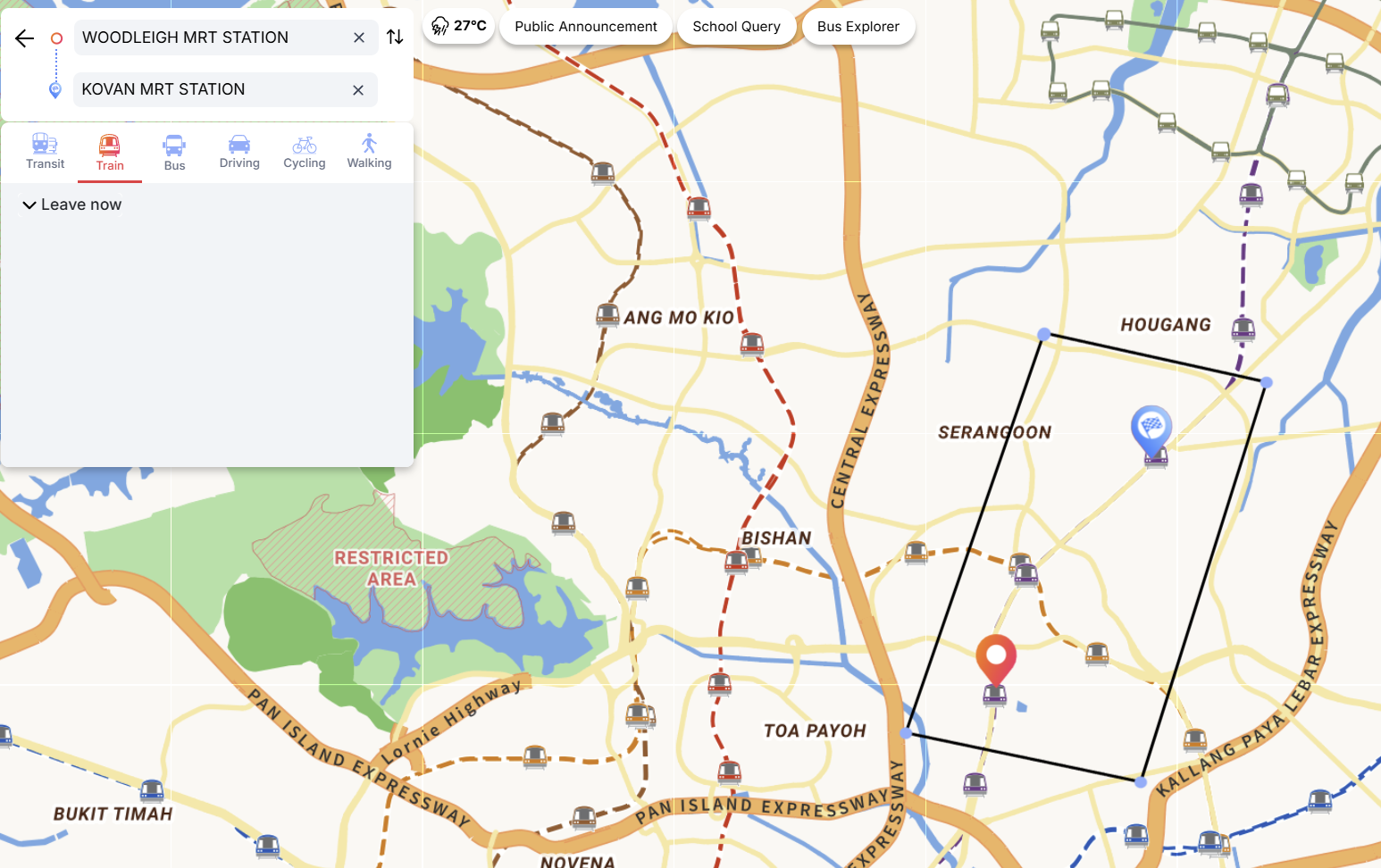
5. Establishing North East Geographical Corridor for analysis

🤦🏻Error in retrieving third query due to missing API token

url = "https://www.onemap.gov.sg/api/common/elastic/search?searchVal=kovan mrt&returnGeom=Y&getAddrDetails=N" response = requests.get(url) print(response.status_code) print(response.json())

• Need API key, see documentation: https://www.onemap.gov.sg/apidocs/authentication

# Retrieve access token (expires 23 Jun 26)
auth_url = "https://www.onemap.gov.sg/api/auth/post/getToken"
payload = {"email": onemap_email, "password": onemap_password}

auth_response = requests.post(auth_url, json=payload)
token = auth_response.json()["access_token"]

headers = {"Authorization": token}

stations = ["kovan mrt", "serangoon mrt", "woodleigh mrt"]
station_coords = {}

for station in stations:
    url = f"https://www.onemap.gov.sg/api/common/elastic/search?searchVal={station}&returnGeom=Y&getAddrDetails=N"
    response = requests.get(url, headers=headers)
    results = response.json()["results"]
    
    station_coords[station] = (results[0]["LATITUDE"], results[0]["LONGITUDE"])

print(station_coords)

{'kovan mrt': ('1.35990191952976', '103.884494725197'), 'serangoon mrt': ('1.3510482896351', '103.871070417199'), 'woodleigh mrt': ('1.33982824592182', '103.87096088798')}

Decision to draw rectilinear bounding box for data analysis around selected corridor (avoid over-engineering for mini project)

Determine min-latlong, max-latlong so rectinlinear boundary can be formed using pandas For future ref Using hulls, Ref1 Shapely lib, Ref2

# Checking dtype in station_coords
for station, coords in station_coords.items():
    print(station, type(coords[0]), type(coords[1]))

kovan mrt <class 'str'> <class 'str'>
serangoon mrt <class 'str'> <class 'str'>
woodleigh mrt <class 'str'> <class 'str'>

lats = [float(coords[0]) for coords in station_coords.values()]
longs = [float(coords[1]) for coords in station_coords.values()]

lats # verify all values are now floats

[1.35990191952976, 1.3510482896351, 1.33982824592182]

longs # verify all values are now floats

[103.884494725197, 103.871070417199, 103.87096088798]

Takeaways:

• station_coords is a dictionary with 3 key-value pairs, 1 for ea station
• .values() pulls out ea stn's tuple at a time, while coord[x] signals for x column
• float() is necy to ensure min-max calcs can be performed (Source)

# Calculate min and max
min_lat = min(lats)
max_lat = max(lats)
min_long = min(longs)
max_long = max(longs)

print(f"Min Latitude: {min_lat}")
print(f"Max Latitude: {max_lat}")
print(f"Min Longitude: {min_long}")
print(f"Max Longitude: {max_long}")

Min Latitude: 1.33982824592182
Max Latitude: 1.35990191952976
Min Longitude: 103.87096088798
Max Longitude: 103.884494725197

Observation 🤔

• For filtering logic: since | gives union, & gives intercept ...
  • Must use & so that a bus stop coordinate falls within each of the 4 min-max-lat-long coords to be considered being IN the cooridor

# finally... the geo-filter we've been waiting for
in_corridor = (
    (merged_clean['Latitude'] >= min_lat) &
    (merged_clean['Latitude'] <= max_lat) &
    (merged_clean['Longitude'] >= min_long) &
    (merged_clean['Longitude'] <= max_long) 
)

# the final filtered corridor as a separate copy - yaY
corridor_df = merged_clean[in_corridor].copy()

# verify final rows we're working with 👀😋
print(corridor_df.shape)

(1278, 12)

🥡Take-away🥢

• Use column names (more fwd looking) in the event dfs are manipulated later down the road (i.e. loc/iloc not so helpful here)
• in_corridor dets which coords in merged_clean satisfy earlier filtering logic
• merged_clean in corridor_df function as a mask, similar to NaN

# random check to ensure road names l00k correct based on domain knowledge 
corridor_df[['RoadName', 'Description', 'Latitude', 'Longitude']].drop_duplicates().head(15)

	RoadName	Description	Latitude	Longitude
132044	Upp S'goon Rd	Aft Bartley Rd	1.341963	103.870969
132404	Bidadari Pk Dr	Opp Blk 212	1.341770	103.875484
132441	Bidadari Pk Dr	Blk 212	1.341638	103.874179
132561	Upp Paya Lebar Rd	Aft Bartley Rd	1.342135	103.883451
132600	Upp Paya Lebar Rd	Aft Rochdale Rd	1.342157	103.884053
132635	Upp Paya Lebar Rd	Wisma AUPE	1.343689	103.882507
132676	Upp Paya Lebar Rd	Paya Lebar Gdns	1.344113	103.882735
132715	Upp Paya Lebar Rd	Bef How Sun Rd	1.345210	103.881710
132757	Upp Paya Lebar Rd	Raya Gdn	1.346768	103.880912
132799	Upp Paya Lebar Rd	Opp Bethany Presby Ch	1.348383	103.880185
132837	Upp Paya Lebar Rd	Aft Paya Lebar Cres	1.349040	103.880227
132879	Upp Paya Lebar Rd	Aft Jln Chermat	1.351704	103.877755
132919	Upp Paya Lebar Rd	Blk 161	1.351701	103.878596
132959	Bartley Rd	Aft Upp Paya Lebar Rd	1.341751	103.881765
133001	Bartley Rd	Bef Upp Paya Lebar Rd	1.341899	103.881654

# Study statistical summary to btr understand spread
corridor_df.groupby('BusStopCode')['TIME_PER_HOUR'].nunique().describe()

count    63.000000
mean     20.285714
std       0.771019
min      18.000000
25%      20.000000
50%      20.000000
75%      21.000000
max      21.000000
Name: TIME_PER_HOUR, dtype: float64

Observation 🤔

• 63 unique buses suggests that there are about 20.285 rows p/bus stop on average.
• Min of 18 service hrs with a max of 21. This differs from earlier basis of 24 hrs of recorded service hrs p day.

# Checking unique hours found in TIME_PER_HOUR column
sorted(corridor_df['TIME_PER_HOUR'].unique())

[np.float64(0.0),
 np.float64(1.0),
 np.float64(5.0),
 np.float64(6.0),
 np.float64(7.0),
 np.float64(8.0),
 np.float64(9.0),
 np.float64(10.0),
 np.float64(11.0),
 np.float64(12.0),
 np.float64(13.0),
 np.float64(14.0),
 np.float64(15.0),
 np.float64(16.0),
 np.float64(17.0),
 np.float64(18.0),
 np.float64(19.0),
 np.float64(20.0),
 np.float64(21.0),
 np.float64(22.0),
 np.float64(23.0)]

Observation 🤔

• Hours 2–4am are absent across the corridor, consistent with most regular bus services terminating by midnight–1am, with only select Night Rider services operating in the deep overnight period (not captured here)
• Can now expect that recorded, filtered data will have 18-21 hr service hour range for buses

corridor_df.groupby('BusStopCode')['TOTAL_TAP_IN_VOLUME'].sum().sort_values(ascending=False).head(10)

BusStopCode
66351    217652.0
66009    206179.0
66359    128172.0
62131     68923.0
66371     44516.0
66051     41415.0
62139     39352.0
66381     35691.0
62059     32562.0
62221     26921.0
Name: TOTAL_TAP_IN_VOLUME, dtype: float64

corridor_df.head(10)

	BusStopCode	RoadName	Description	Latitude	Longitude	YEAR_MONTH	DAY_TYPE	TIME_PER_HOUR	PT_TYPE	PT_CODE	TOTAL_TAP_IN_VOLUME	TOTAL_TAP_OUT_VOLUME
132044	61049	Upp S'goon Rd	Aft Bartley Rd	1.341963	103.870969	2026-05	WEEKDAY	22.0	BUS	61049.0	156.0	294.0
132045	61049	Upp S'goon Rd	Aft Bartley Rd	1.341963	103.870969	2026-05	WEEKDAY	15.0	BUS	61049.0	346.0	615.0
132046	61049	Upp S'goon Rd	Aft Bartley Rd	1.341963	103.870969	2026-05	WEEKDAY	6.0	BUS	61049.0	977.0	331.0
132047	61049	Upp S'goon Rd	Aft Bartley Rd	1.341963	103.870969	2026-05	WEEKDAY	5.0	BUS	61049.0	223.0	86.0
132050	61049	Upp S'goon Rd	Aft Bartley Rd	1.341963	103.870969	2026-05	WEEKDAY	23.0	BUS	61049.0	107.0	127.0
132052	61049	Upp S'goon Rd	Aft Bartley Rd	1.341963	103.870969	2026-05	WEEKDAY	7.0	BUS	61049.0	1675.0	708.0
132057	61049	Upp S'goon Rd	Aft Bartley Rd	1.341963	103.870969	2026-05	WEEKDAY	9.0	BUS	61049.0	987.0	471.0
132059	61049	Upp S'goon Rd	Aft Bartley Rd	1.341963	103.870969	2026-05	WEEKDAY	0.0	BUS	61049.0	29.0	32.0
132060	61049	Upp S'goon Rd	Aft Bartley Rd	1.341963	103.870969	2026-05	WEEKDAY	10.0	BUS	61049.0	557.0	255.0
132061	61049	Upp S'goon Rd	Aft Bartley Rd	1.341963	103.870969	2026-05	WEEKDAY	18.0	BUS	61049.0	690.0	1103.0

C. Exploratory Data Analysis: Plotting

6. Plotting high-density bus stops

• Sum of (tap-in + tap-out) across all hours, grouped by bus stops = total passenger volume

corridor_df['total_volume'] = corridor_df['TOTAL_TAP_IN_VOLUME'] + corridor_df['TOTAL_TAP_OUT_VOLUME']

stop_volume = (
    corridor_df
    .groupby(['BusStopCode', 'Description'], as_index=False)['total_volume']
    .sum()
    .sort_values('total_volume', ascending=False)
)

# Plot 1: Top 5 vs Bottom 5 Corridor Bus Stops by Total Passenger Volume 
import matplotlib.pyplot as plt
import matplotlib.colors as mcolors
import seaborn as sns
import folium
from folium.plugins import HeatMap
import base64
from io import BytesIO
from IPython.display import HTML, display

# Filtering desired rows
top5 = stop_volume.head(5)
bottom5 = stop_volume.tail(5)
plot_df = pd.concat([top5, bottom5])

# Colour mapping
norm = mcolors.Normalize(vmin=plot_df['total_volume'].min(), # rescales volume numbers into 0-1 range for cmap reading
                         vmax=plot_df['total_volume'].max())
cmap = mcolors.LinearSegmentedColormap.from_list("custom_blue_red", ["#2c7da0", "#e63946"])  # blue (low) to red (high), monotonic
bar_colors = [cmap(norm(v)) for v in plot_df['total_volume']] # unique col p/bar

# Plot dimensions 
fig, ax = plt.subplots(figsize=(12, 8))

# Plot + annotations (annotations depend on the plotted bars existing)
sns.barplot(data=plot_df, 
            x='Description', 
            y='total_volume', 
            hue='Description',
            palette=bar_colors, # unique col p/bar
            legend=False, 
            ax=ax)
for container in ax.containers:
    ax.bar_label(container, 
                 fmt='%.0f', 
                 color='white', 
                 padding=3, 
                 fontsize=9)
# Grid behind plots
ax.grid(axis='y', 
        color='white', 
        alpha=0.3, 
        zorder=0)
ax.set_axisbelow(True)  

# Styling
fig.patch.set_facecolor('#1e1e1e')
ax.set_facecolor('#1e1e1e')
ax.set_xticks(ax.get_xticks())
ax.set_yticks(ax.get_yticks())
ax.tick_params(axis='both', colors='white', labelsize=7)
plt.setp(ax.get_xticklabels(), rotation=45, ha='right')
ax.set_ylabel('Total Passenger Volume (Tap-In + Tap-Out)', color='white')
ax.set_xlabel('Bus Stop', color='white', fontsize=10)
ax.set_title('Not All Stops Are Equal', color='white', fontsize=18)
plt.tight_layout()

# Export to base64 PNG for side-by-side HTML layout
buf = BytesIO()
fig.savefig(buf, format='png', dpi=120)
plt.close(fig)
buf.seek(0)
img_b64 = base64.b64encode(buf.read()).decode('utf-8')


# Accompanying Folium map: Top 5 vs Bottom 5 bus stops, plus 3 MRT stations
top5_codes = top5['BusStopCode'].tolist()
bottom5_codes = bottom5['BusStopCode'].tolist()
marker_codes = top5_codes + bottom5_codes

map_df = stop_volume[stop_volume['BusStopCode'].isin(marker_codes)].merge(
    corridor_df[['BusStopCode', 'Latitude', 'Longitude']].drop_duplicates('BusStopCode'),
    on='BusStopCode'
)

mrt_stations = {
    'Kovan MRT': (1.3602, 103.8849),
    'Serangoon MRT': (1.3499, 103.8731),
    'Woodleigh MRT': (1.3392, 103.8708),
}

center_lat = map_df['Latitude'].mean()
center_lon = map_df['Longitude'].mean()
m = folium.Map(location=[center_lat, center_lon], zoom_start=14, tiles='CartoDB voyager')

heat_data = [[row['Latitude'], 
              row['Longitude'], 
              row['total_volume']] for _, row in map_df.iterrows()] # weight = glow intensity affected by passenger vol
HeatMap(heat_data, radius=35, blur=15, max_zoom=14).add_to(m) # controlling glow spread

for _, row in map_df.iterrows():
    color = mcolors.to_hex(cmap(norm(row['total_volume'])))
    folium.CircleMarker(
        location=[row['Latitude'], row['Longitude']],
        radius=10,
        popup=f"{row['Description']}: {int(row['total_volume']):,} pax",
        color=color,
        fill=True,
        fill_opacity=0.8
    ).add_to(m)

for name, (lat, lon) in mrt_stations.items():
    folium.CircleMarker(
        location=[lat, lon],
        radius=10,
        popup=name,
        color='#1d3557',
        fill=True,
        fill_color='#457b9d',
        fill_opacity=0.9
    ).add_to(m)

# Collect all coordinates to fit bounds (bus stops + MRT stations) 
all_coords = [[row['Latitude'], row['Longitude']] for _, row in map_df.iterrows()]
all_coords += [[lat, lon] for lat, lon in mrt_stations.values()]

m.fit_bounds(all_coords)  # set initial view to fit everything

# Recenter button: call Leaflet's fitBounds() on the map's JS object 
recenter_button = f"""
<button onclick="{m.get_name()}.fitBounds({all_coords});"
        style="position:absolute; top:10px; right:10px; z-index:9999;
               padding:6px 12px; background:white; border:1px solid #999;
               border-radius:4px; cursor:pointer; font-size:13px;">
  Recenter
</button>
"""
m.get_root().html.add_child(folium.Element(recenter_button))

map_render = m.get_root().render().replace(chr(34), "&quot;")
map_html = f'<iframe srcdoc="{map_render}" style="width:100%; height:700px; border:none;"></iframe>'

# Configuration for side by side display
combined = f"""
<div style="display: flex; align-items: flex-start; gap: 10px;">
    <div style="flex: 0.65; height: 700px;">
        <img src="data:image/png;base64,{img_b64}" style="height:100%; width:auto; max-width:100%; object-fit:contain;">
    </div>
    <div style="flex: 0.35; height: 700px;">
        {map_html}
    </div>
</div>
"""
display(HTML(combined))

Figure 1: Tap-in vs tap-out, top 5 stops — Serangoon Stn dominates total footfall.

Plot 1 analysis

• Top 5 highest-vol stops range between 100,000 to 350,000 taps
• Bottom 5 lowest-vol stops have extremely scarce daily ridership (Quick math: 109 to 71 passengers on daily average for 31-day May)
• Highest-vol stops congregate around rail access point ~ primarily Serangoon station, and interestingly not at the other two stations.
  • Could also suggest greater residential density around that particular region, given that the full list of bus stops fall within a corridor containing 3 stations.

7. Plotting inbound and outbound journeys

# Plot 2: Tap-In vs Tap-Out for Top 5 NE Corridor Bus Stops by Total Monthly Passenger Volume

# Data prep: Narrowing Top 5 highest-vol stops and converts from Pandas Series into Python list
top5_codes = stop_volume.head(5)['BusStopCode'].tolist()

# Data prep:
direction_df = (
# .isin() filters Top5 BusStopCode's row from corridor_df using True/False
    corridor_df[corridor_df['BusStopCode'].isin(top5_codes)]
# Groupby 2 select columns, displaying tap-in, tap-out data side-by-side
    .groupby(['BusStopCode', 'Description'], as_index=False)[['TOTAL_TAP_IN_VOLUME', 'TOTAL_TAP_OUT_VOLUME']]
# Totalling all taps in/out
    .sum()
# merging the total_volume column with the BusStopCode column
    .merge(stop_volume[['BusStopCode', 'total_volume']], on='BusStopCode')
# Sort by overall size
    .sort_values('total_volume', ascending=False)
)

# .melt() reshapes from "one row p/stop, two separate columns" to "one row p/stop p/direction"
direction_long = direction_df.melt(
    id_vars=['Description'],
    value_vars=['TOTAL_TAP_IN_VOLUME', 'TOTAL_TAP_OUT_VOLUME'],
    var_name='Direction',
    value_name='Volume'
)
direction_long['Direction'] = direction_long['Direction'].map({
    'TOTAL_TAP_IN_VOLUME': 'Tap-In',
    'TOTAL_TAP_OUT_VOLUME': 'Tap-Out'
})

# Colour mapping — same icefire colormap as Plot 1, pulled at two contrasting points
icefire_cmap = sns.color_palette("icefire", as_cmap=True)
palette = [icefire_cmap(0.15), icefire_cmap(0.85)]  # blue end, orange/red end

# Plot dimensions
fig, ax = plt.subplots(figsize=(15, 6))
fig.patch.set_facecolor('#1e1e1e')
ax.set_facecolor('#1e1e1e')

# Plot + annotations
sns.barplot(data=direction_long, x='Description', y='Volume', hue='Direction', palette=palette, ax=ax)
for container in ax.containers:
    ax.bar_label(container, fmt='%.0f', color='white', padding=3, fontsize=9)
ax.grid(alpha=0.2)
ax.set_xticks(ax.get_xticks())
ax.set_yticks(ax.get_yticks())
ax.tick_params(axis='both', colors='white', labelsize=9)

# Styling: labels + layout
ax.set_xlabel('Bus Stop Names', fontsize=12, color='white')
ax.set_ylabel('Total Weekday Volume (May 2026)', fontsize=12, color='white')
ax.set_title('Coming or Going? Tap-in and Tap-out Patterns at the Top 5 Stops', fontsize=20, color='white')

# Legend styling
legend = ax.legend(title='Direction')
legend.get_frame().set_facecolor('#1e1e1e')
legend.get_frame().set_edgecolor('white')
for text in legend.get_texts():
    text.set_color('white')
legend.get_title().set_color('white')

plt.tight_layout()
plt.show()

Figure 2: Tap-In vs Tap-Out for Top 5 NE Corridor Bus Stops by Total Monthly Passenger Volume.

Plot 2 analysis

• [Arrival Points] Serangoon Station Exit C/Blk 201, and Serangoon Station Exit A/Blk 413
  • For former, tap-out (227,744) far exceeds tap-in (128,172) indicates strong in-flow (perhaps corridor outbound) -> perhaps multi-modal journey (i.e. bus-train)
  • Simliar for latter
• [Departure Points] Serangoon Station Exit E, Serangoon Interchange, and Serangoon Station Exit B
  • The reverse is observed, where tap-in exceeds tap-out indicates outflow (perhaps corridor inbound) -> perhaps multi-modal journey (i.e. train-bus)

8. Plotting congestion across an average weekday

# Plot 3: Passenger Flows Per Hour on an Average Weekday at Top 3 NE Corridor Bus Stops
from matplotlib.patches import Patch # generic matplotlib shape object

# Data prep: Grabbing Top 3 highest-vol stops and converts from Pandas Series into Python list
top3_codes = stop_volume.head(3)['BusStopCode'].tolist()

# Data prep: 
hourly_top3 = (
# .isin() filters Top3 BusStopCode's row from corridor_df using True/False
    corridor_df[corridor_df['BusStopCode'].isin(top3_codes)]
# Groupby 3 select columns, incl. Time P/H for study
    .groupby(['BusStopCode', 'Description', 'TIME_PER_HOUR'], as_index=False)['total_volume']
    .sum()
    .sort_values('TIME_PER_HOUR')
)

# Colour mapping
icefire_cmap = sns.color_palette("icefire", as_cmap=True)
line_colors = [icefire_cmap(0.1),   # light blue 
               icefire_cmap(0.25),  # cool blue
               icefire_cmap(0.8)]   # warm -> highest congestion

# Plot dimensions
fig, ax = plt.subplots(figsize=(15, 6))
# Grey bg for plot
fig.patch.set_facecolor('#1e1e1e')
ax.set_facecolor('#1e1e1e')

# Plot of Top 3 highest-vol bus stops
sns.lineplot(data=hourly_top3, 
             x='TIME_PER_HOUR', 
             y='total_volume', 
             hue='Description', # groups lines by bus stop name
             palette=line_colors, # ensures each grouped line has distinct colour
             marker='o', 
             ax=ax)
# Highlighting the congestion windows
ax.axvspan(6,            # AM peak window
           9, 
           color='yellow', 
           alpha=0.25)   
ax.axvspan(17,           # PM peak window
           20, 
           color='yellow', 
           alpha=0.10)  

# Grid behind plots
ax.grid(alpha=0.2, 
        color='white', 
        zorder=0)
ax.set_axisbelow(True)

# Styling
ax.set_xticks(range(0, 24))
ax.set_yticks(ax.get_yticks())
ax.tick_params(axis='both', 
               colors='white', 
               labelsize=9)
ax.set_xlabel('Hour of Day', 
              color='white', 
              fontsize=12)
ax.set_ylabel('Total Passenger Volume (Tap-In + Tap-Out)', 
              color='white', 
              fontsize=12)
ax.set_title('Rush hours: Passenger Flows at the Top 3 NE Corridor Stops (May 2026)',
             color='white', 
             fontsize=18)

# Legend styling 
peak_patch = Patch(facecolor='yellow', # define shape object's properties fir AM/PM peak
                   alpha=0.2, 
                   label='Peak Hours (AM/PM)')
handles, labels = ax.get_legend_handles_labels() # 3 Line2D objects representing each stop + text labels
handles.append(peak_patch) # adding AM/PM peak to legend
labels.append('Peak Hours (AM/PM)') 
legend = ax.legend(handles=handles, # setting up legend with our defined properties
                   labels=labels, 
                   title='Legend',
                    bbox_to_anchor=(1.02, 1), 
                   loc='upper left')

legend.get_frame().set_facecolor('#1e1e1e') # setting up legend frame 
legend.get_frame().set_edgecolor('white')
for text in legend.get_texts():
    text.set_color('white')
legend.get_title().set_color('white')

plt.tight_layout()
plt.show()

Figure 3: Passenger Flows Per Hour on an Average Weekday at Top 3 NE Corridor Bus Stops.

Plot 3 analysis

• The morning peak window has more extreme changes in passenger volume compared to the evening peak window
• The three bus stops have quite starkly different passenger volumes in the morning, with Serangoon Station Exit C/Blk 201 having the highest change
• The three bus stops have a similar rise-fall flow during the evening peak window
• Worth noting that both red & cool blue bus stops are connected to the North East MRT line, and the light blue is connected to a bus interchange.

9. Plotting distribution of passenger volume across 63 bus stops

# Plot 4: Distribution of Total Weekday Passenger Volume across 63 Corridor Bus Stops

# Colour mapping 
icefire_cmap = sns.color_palette("icefire", 
                                 as_cmap=True)
box_color = icefire_cmap(0.20)    # cool end, for the box itself
point_color = icefire_cmap(0.95)  # warm end, visible against dark bg, distinct from box

# Plot dimensions
fig, ax = plt.subplots(figsize=(8, 8))
# Grey bg for plot
fig.patch.set_facecolor('#1e1e1e')
ax.set_facecolor('#1e1e1e') 

# Plot
# Box: IQR + Median
sns.boxplot(y=stop_volume['total_volume'], 
            color=box_color, 
            width=0.3, 
            ax=ax, 
            showfliers=False)
# 63 bus stops 
sns.stripplot(y=stop_volume['total_volume'], 
              color=point_color, 
              alpha=0.6, 
              size=4, 
              jitter=True, 
              ax=ax)
# Grid behind plots
ax.grid(axis='y', 
        alpha=0.2, 
        color='white', 
        zorder=0)
ax.set_axisbelow(True)

# Styling
ax.set_yticks(ax.get_yticks())
ax.tick_params(axis='both', 
               colors='white', 
               labelsize=9)
ax.set_ylabel('Total Passenger Volume (Tap-In + Tap-Out)', 
              color='white', 
              fontsize=12)
ax.set_title('Three Stops Carrying the North Eastern Corridor',
             color='white', 
             fontsize=13)

plt.tight_layout()
plt.show()

# Identifying 3 outliers
stop_volume.nlargest(3, 'total_volume')[['Description', 'total_volume']]

	Description	total_volume
56	S'goon Stn Exit C/Blk 201	355916.0
55	S'goon Stn Exit E	331501.0
52	Serangoon Int	309944.0

Figure 4: Distribution of Total Weekday Passenger Volume across 63 Corridor Bus Stops.

Plot 4 analysis

• Three stops carry disproportionately high volume relative to the rest of the North East Corridor

D. Conclusion

10. Answering the RQ:

• Load is highly uneven across the north eastern corridor, particularly at the bus stops surrounding Serangoon
  • evidenced by Plot 1 (vol conc + Folium map), Plot 4 (distribution)
• While included in the dataset, bus stops surrounding Kovan and Woodleigh didn't make it to the Top or Bottom.
• For the bottom stops that still fall within Serangoon's catchment with minimal traffic
  • proximity to Serangoon alone doesn't predict volume: these stops are 240 – 840m from the MRT, while the top 5 are 0m from station exits
  • this suggests volume concentration is driven by direct rail-transfer function , not just geographic nearness to the station
• Plot 2 and 3 enable deeper forensic understanding of congestion in that we are able to determine direction (inbound/outbound imbalance for former), and time window peaks. Both shed light into where bus-rail systems require greater integration for smoother transfers (i.e. increased turnover, lower waiting times, more ground staff deployments...etc.)

Passenger load concentrates sharply around Serangoon's MRT station exits, with comparatively little signal of bus-rail integration at Kovan or Woodleigh MRT stations

So what?

• Serangoon's bus passenger volume data provides insight into what bus-rail integration needs are, and where gaps might need to be plugged.
• Comparisons with other equally loaded corridors is likely to lead to greater learning, and clearer evaluation of LTMP 2040's policy effectiveness.

Limitations of study

• These analyses were based on a single month of data collection in May 2026 for weekdays only.
• Only looked at bus passenger volume, and examining rail passenger volume in tandem would enable more thorough analysis.

References & Acknowledgements

I would like to thank Dr Chaitanya Rao, my Institute of Data course instructor, as well as Rachel Anastasi-Marais, our course teaching assistant, for their invaluable help and coaching throughout the course so far. None of these developing data analytical skills would have been possible within a condensed timeframe without their encouragement and skills building tutoring.

Many thanks to the LTA Datamall team for their help in solving a silly API key-access blip so I could more readily access the rich store of data made ready to the public for such analytical projects. I am also grateful for access to URA's OneMap, whose interactive features made intuitively figuring out a geographical boundary for EDA a lot easier for manipulating with Pandas's coding logic.

Disclaimer:

The observations and take-aways expressed in this notebook are for the purposes of personal data exploration and analysis.

Show Code